Grade 1

• The triangle.
• Pythagoras’s Theorem.
• Simple trigonometry.

Grade 2

• Theodorus Spiral
• What is Pi?
• Computer programming: Matlab and Python.
• Data visualisation.

Grade 3

• Pattern recognition.

---

Grade 1

Step 1.  The First Triangle

This is a triangle:

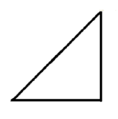
Can you see this triangle has two sides with the same length?

Between the sides there are angles (measured in degrees (°).

This triangle is called a Right Isosceles Triangle because it has two sides of equal length and it has a 90° angle which is also called a right angle.

If we call the sides (adjacent, opposite and hyptenuse) like this::

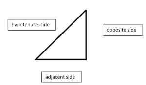
and give the adjacent and opposite values of one (1).

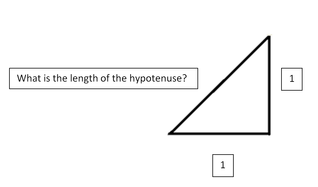
To answer the question, “what is the length of the hypotenuse?”,
you need to use Pythagoras’s Theorem.

Step 2. Pythagorus’s Theorem

A right angled triangle is used in Pythagoras’s Theorem
(the other sides and angles do not need to be equal).

If we draw squares out from the sides of the right angle triangle and understand that the length of a side of a square multiplied by itself is the area. The equation convention for ‘squaring’ is written with a raised little two .

Then call one of the shorter sides ‘a’ and the other ‘b’ and  the longest side ‘c’.  Add the two smaller areas and this is the area of the biggest square.

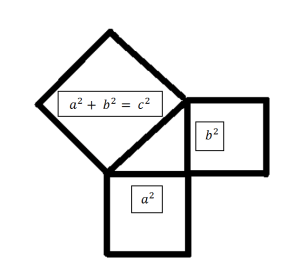
Rearrange the equation to find the length of side ‘c’ by calculating the ‘square root’:

Back to the triangle:

What is the length of the hypotenuse if the adjacent side and the opposite side are equal to one?

√2 is equal to 1.4142135 (this number keeps going) and is an irrational number.

Step 3. Simple trigonometry

Finding the other angles:

This is the first triangle in the Theodorus Spiral

Grade 2

Step 4. The Spiral of Theodorus

If each successive hypotenuse become the next adjacent length and the opposite length remains 1 and the each triangle a right triangle (no longer an isosceles triangle) we get the Theodorus Spiral:

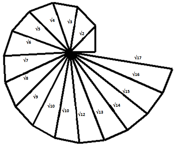
This figure was created using the following Matlab computer code:

Notes:   in computer coding         is writting sqrt(x)

clear all
total_angle=0;
winding=0;

fprintf('  x        hyp         X          Y           winding \n');

for x=1:16

hyp=sqrt(x+1);
angle=atan(1/sqrt(x));
total_angle=total_angle+angle;
X=hyp*cos(total_angle);
Y=hyp*sin(total_angle);
degtotal_angle=total_angle*180/pi;
winding=degtotal_angle/360;

hypb=sqrt(x);
Xb=hypb*cos(total_angle-angle);
Yb=hypb*sin(total_angle-angle);


hold on
plot ([0 1],[0 0],'k','LineWidth',3);    %first spoke
plot ([0 X],[0 Y],'k','LineWidth',3);    %spokes
plot ([Xb,X],[Yb Y],'k','LineWidth',3);  %boundary

fprintf('%3i  %10f   %10f   %10f   %10f  \n',x , hyp, X,Y, winding);

end